Breaking down factors of Covid-19 orientation algorithm by importance
Computing variable importances: Sobol Indices, Shapley Effects and Shap
Let’s 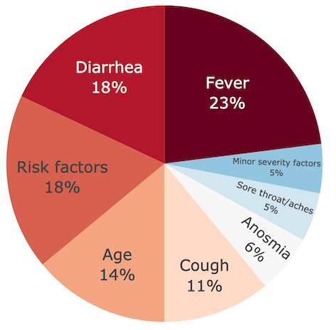 dig deeper on the important factors of the French Covid-19 patient orientation algorithm!
The short answer is fever, diarrhea and number of risk factors, but the real answer is that your target population matters a lot.
dig deeper on the important factors of the French Covid-19 patient orientation algorithm!
The short answer is fever, diarrhea and number of risk factors, but the real answer is that your target population matters a lot.
Follow me on this journey with 3 variable importance methods and get some insights about how factors interact.
If you are in a hurry, go and see the take-away messages or have a look at the python code.
Context and objectives
You are a user of a complex decision process, a black box predictive model, an unknown algorithm. Wouldn’t you be glad to see a summary of how much different variables impact the outcome? With these importances in hand, you have a better understanding on how this model behaves. Furthermore, you better see how two algorithms differently weight the inputs.
You build or have advanced access to an algorithm or a complex model. Wouldn’t you be reassured to verify that inputs that should matter, really matter in your model? Moreover, you can use it for factor prioritization and spend time on variables that counts. And think of the users, don’t they deserve an overview of what’s important?
In this post, we will talk about methods to compute factor importances (also called variable importances). After a detour by the Sensitivity Analysis community - overlooked by too many data scientists, I will quickly present the 3 methods used: Sobol indices, Shapley Effects and shap Importances. Finally, the results are presented and discussed, on a simplified version on the French Covid-19 orientation algorithm. If you don’t know it, you should check this section of my previous post, which presents and simplifies it into a scoring system version.
Approaches in literature
Extracting importances from variables is one of the focus of the Sensitivity Analysis in Statistics. A good introduction is the 2015 successful paper1, where 2 French researchers -Iooss and Lemaître- reviewed the main Global Sensitivity analysis methods. They group these techniques by their goal, into 3 categories: screening (coarse sorting of the most influential inputs among a large number), measures of importance (quantitative sensitivity indices) and deep exploration of the model behaviour (measuring and viewing the effects of inputs on their all variation range).
Our focus here is of course the second category (measure of variable importance), i.e. computing values which tell how much input variables (factors) contribute to an interest quantity depending on model output. We will use several techniques borrowed from different fields:
- From Sensitivity Analysis field (Uncertainty Quantification):
- Sobol Indices (Total-order)
- Shapley Effects
- From the recent Explainable AI (XAI) field: shap Importances (KernelShap).
Importances need context!
Before going into method specifics, there is an important point to talk about.
Should the factor importances depend on the probability distribution of each factor?
For example, should the importance of the number of minor severity factors depend on the proportion of older people (vs younger)?
Remember that they interact in the following way in our equivalent scoring system:
If 0 minor severity factor AND age < 50y then +0pt else +6pts.
Let's think. If there are only young people, severity factors starts to matter a lot because it becomes the only driver to tip from +0pt to +6pts. Reversely, with only older people, severity factors don't matter anymore because the outcome will be +6pts, whatever the NMSF.Yes, factor importances do depend on factors distributions, even if they are independent. Here are the main two reasons:
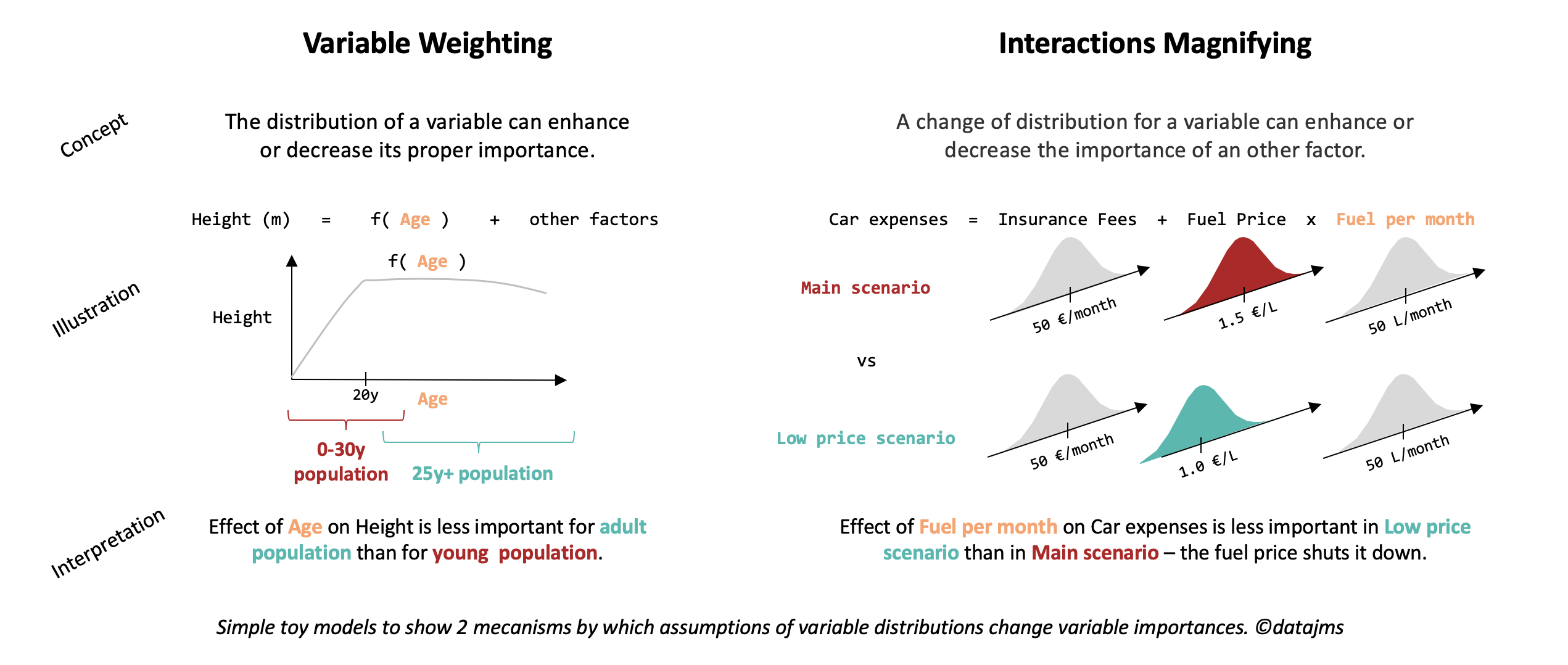
- Variable Weighting: the distribution of a factor could enhance or fade out its proper importance. Let’s imagine that we study the importance of age and other factors in the height of human (see figure below). On a young population, we expect age to predominate ; while with grown-up adults, other factor would be the most important.
- Interactions Magnifying: as illustrated in the severity factors-age example above or in the car expenses illustration below, a distribution shift can enhance or fade out the importance of an other factor, when there are strong interactions in the model.
Application to Covid-19 orientation algorithm
Assumptions
Here are the assumptions, for the rest of the analysis:
- Restriction to Tele-consultation vs No action scope.
We know that having a major severity factor is the one and only condition for the outcome Call emergency.
So the major severity factors would have the largest importance, assuming that there is no extreme fading variable weighting effect.
So, we exclude both variable Major severity factors and outcome Call emergency from the analysis and focus on the remaining 8 binary variables for the Tele-consultation vs No action algorithm. - Two scenarios of factor distribution: as mentioned previously, choosing a distribution of factors is a pre-requisite to compute importances.
We first assume here the independence of all variables, which is actually a strong assumption, but note that Shapley Effects method handles dependent variables.
Then we build 2 scenarios of distribution:
A, a pseudo-realistic scenario which avoid too much Variable Weighting effect (all proportions are equal to 20%, except for age), and B, a scenario where all categories are equiprobable.
When discussing results below, a section is dedicated to compare these 2 scenarios.
| Scenario | Age | Anosmia | Cough | Diarrhea | Fever | Number of minor severity factors |
Number of risk factors |
Sore throats/aches |
|---|---|---|---|---|---|---|---|---|
| A | 50% <50y, 50% ≥50y |
20% yes, 80% no |
20% yes, 80% no |
20% yes, 80% no |
20% yes, 80% no |
20% ≥1, 80% 0 |
20% ≥1, 80% 0 |
20% yes, 80% no |
| B | 50% <50y, 50% ≥50y |
50% yes, 50% no |
50% yes, 50% no |
50% yes, 50% no |
50% yes, 50% no |
50% ≥1, 50% 0 |
50% ≥1, 50% 0 |
50% yes, 50% no |
Sobol Indices
Designed by Sobol in the 90s2, total-order Sobol indices are computed for each factor. They capture the effect of a factor on the outcome, including its interactions with all other variables. The effect of a factor is measured in terms of variance brought by this factor, compared to the total variance of the outcome.
Contrary to what is sometimes believed, the total-order indices don’t necessarily add up to 1. They would do, if all factors were independent (assumption ok here) and if the function were additive, i.e. no interaction term involved. As explicit interactions terms (cough & fever, number of risk factor & age, etc.) appear, we expect the sum to be larger than 1. Results show indeed that the sum of the total Sobol indices is about 1.70 for scenario A and 2.15 for B. To allow method comparisons, we will scale down the indices so that they effectively sum to 1.
The implementation is straightforward with the robust python SALib library, using the sobol.analyze function. The main design choice is the simulation of the factor distributions to create the 2 scenarios. In brief, although our 8 factors are binary, we stick into the SALib framework, use uniform 0-1 distributions and modify the decision function to account for the scenario distributions3.
Shapley Effects
Introduced by Owen in 20144 and extended to correlated factors by Song et al in 20165 and Iooss & Prieur in 20176, Shapley Effects are similar to the total-order Sobol indices. The re-written variance decomposition, with a smart use of shapley values from game theory, ensures that the Shapley Effects add up to 1. Moreover, they can be extended to dependent factors - but this goes beyond the scope of this article.
However, they come at a price: their computation. They require even more model evaluations than Sobol indices. To overcome this drawback, recent 2019 work by Benoumechiara & Elie-Dit-Cosaque7 focuses on providing robust confidence intervals and decrease the number of required model evaluations.
The implementation has been done with the python shapley-effects library (more resources would have been available in the Sensitivity R package). The installation is not straightforward, but I managed to quickly use the different functions8. Scenario A and B were set-up with the same trick than previously for Sobol indices (uniform distribution with an appropriate threshold for the step functions).
shap Importances
Designed and implemented by Lundberg in 20179, shap has an other focus than the previously mentioned variance-based global indices. It is a local feature-attribution method, which aims at attributing the value of a single evaluation (one person getting its Covid-19 recommendation) to the input factors. Therefore, we can write that outcome = attribage + attribcough + … + attribsore_throat + average_outcome_for_population. Outcome is 0 for No action and 1 for Tele-consultation. Each term is different for each person, except average_outcome_for_population. Shapley values are used for weighting so that attributions satisfy consistency properties.
So, shap provides us with a list of factor attributions (called shap values) for each person. To have a global vision, shap Importances are usually10 computed by averaging the absolute value of shap values, over population. To allow method comparisons, we will scale down the shap Importances so that they sum to 1.
The implementation has been done with the python shap library, which is robust and well documented now. We used the KernelShap estimation (KernelExplainer class), which is a bit slow but enough for our 8-variable setting11.
Running simulations
You can have a look at the code used to run the simulations, including the Covid-19 orientation algorithm, importances computation and final plots. For the 2 scenarios, each importance is run 50 times independently, so that we can have an uncertainty bar (spanning from minimum to maximum of the 50 values). With the chosen parameters (not discussed, but you can see the set-up here12), it took approximately ~18h with 3 processes on a dual core 2.3Ghz Intel i5. Sobol index was relatively fast (~20 min with a single process) whereas the other 2 took about the same time.
Results
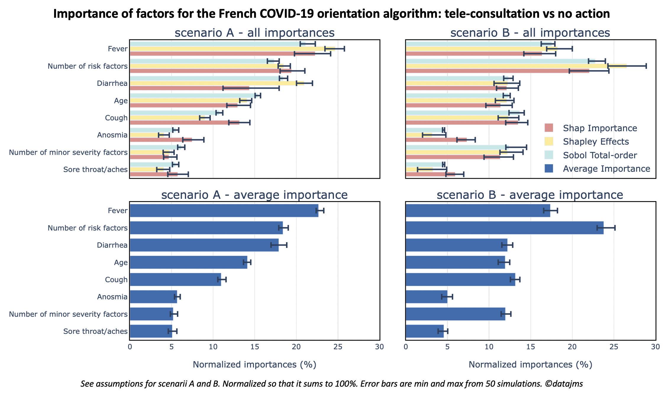
The results of simulations are presented as horizontal bars with error bars, allowing to compare:
- The variations between the 3 importance methods
- The 8 factors of Covid-19 orientation algorithm
- Our 2 scenarios of probability distribution
Each importance type has been normalized (rescaled to sum up to 100%) in the following figures.
Colors show the 3 importance types explained before and Average Importance the average of the 3.
The 3 methods
Overall, the 3 methods give similar importances13 and the 3 ordering wouldn’t be very different from each other. It makes it consistent (very pragmatical, but no theory behind this) to build a summary metrics: the Average Importance. Its definition is straightforward: the average of the 3 normalized importances for each factor.
Concerning the 3 importance methods, some conclusions can be drawn:
- Sobol Indices are the fastest importance method estimation here: they were estimated almost 100 times faster and they still have the lowest error bars.
- shap Importances have less extreme values between factors14.
8 factors discussion
Let’s focus on scenario A first and keep the discussion concerning A vs B for the next part. Under scenario A assumptions, importances between factors give the following ordering of 5 groups of factors: fever (23%), number of risk sactors and diarrhea (18% each), age (14%), cough (11%) and finally the 3 last factors: anosmia, sore throat/aches and number of minor severity factors (5-6% each). A few observations:
- Anosmia and sore throat/aches play a symmetric role in the decision tree. So their importances should be roughly equal, which is indeed the case. Moreover, we rightly expected their importances to be small (as suggested by the equivalent scoring system).
- Fever and number of risk factors were expected as very important variables! However, note that I personally expected cough to play a more important role (especially since its score coefficients differs only by 1pt from fever: +4pts vs +3pts), but more on this in the scenarios comparison.
- Diarrhea and number of minor severity factors were my biggest surprises: I would have expected the former to be less important and the latter not to be in the last position.
- Finally, age is in the middle of the ranking, and I didn’t have strong opinions about it!
To sum-up, the error bars are small enough to result in a robust importance ranking. This ranking was more or less expected. However, some importance factors are surprising: the large difference between fever and cough, the importance of diarrhea and the counter-performance of the number of minor severity factors.
scenarios analysis
The bar plots are clear about it: our scenarios, based on factor probability distribution, play a major role. Moving from scenario A to B, number of minor severity factors and number of risk factors are the biggest winners (more than 5pts of perc. increase), diarrhea and fever the big losers (more than 5pts of perc. decrease) and the stable remaining factors (less than 2pts of perc. change).
Note that going from scenario A to B (see scenario definition) is equivalent to change the 80/20 proportions into 50/50 for each factor (expect age, which remains 50/50).
Therefore and using the concepts introduced before, switching from A to B doesn’t change the variable weighting (except relatively, for age) but increases a lot the interactions magnifying (for 2-term interactions: 0.25 vs 0.04 probability; for 3-term interactions: 0.125 vs 0.008 probability, etc.).
Basically, scenario B puts more weight on interactions between factors and increases importances which rely on strong interactions (the more terms, the more relative weight is added).
With this perspective:
- The big winners make sense. The number of minor severity factors and number of risk factors appears in interactions with at least 3-terms and often 4 terms, so there importances have a boost in scenario B.
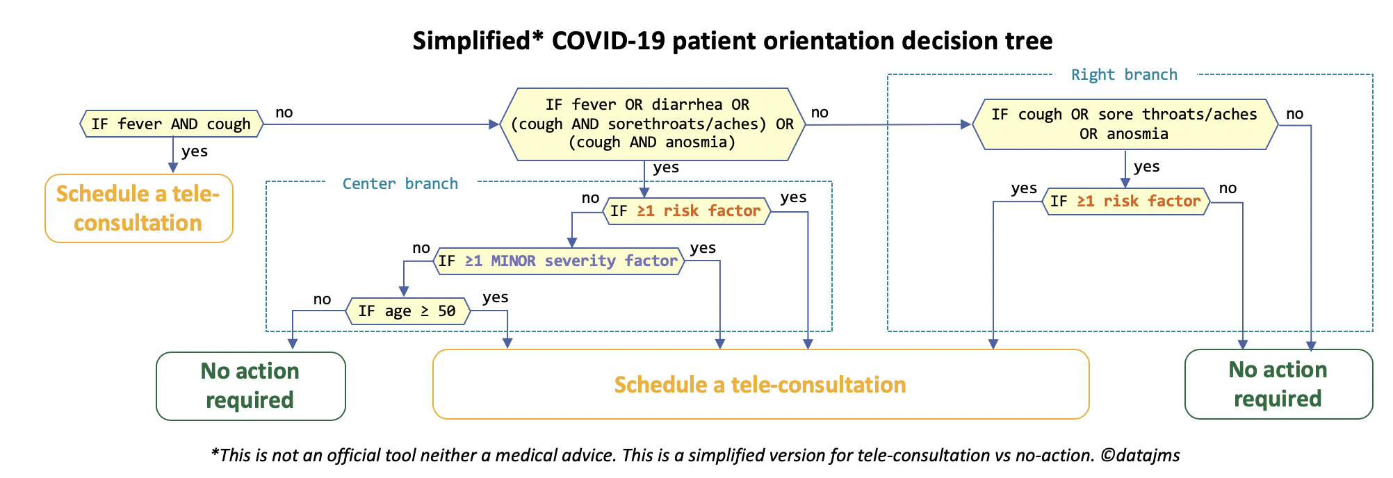
- The big losers (diarrhea and fever) are variables that drives decisions shortly, without long 3-term or 4-term interactions. Let’s focus on diarrhea, who can drive the switch between the center branch and the right branch (see simplified tree above). The strength of diarrhea in scenario A comes from the fact that it is a main driver of the center vs right branch switch (the 2-term interactions of cough are relatively less likely in A) and that this switch matters more in scenario A (bigger outcome probability gap than in B15). Similar explanations exist for fever. So, fever and diarrhea lose relative importance, compared to the big winners from scenario B.
- The 4 stable remaining factors have mixed effects and explanations. For example, in scenario B anosmia and sore throat/aches increase their power in driving the center vs right branch switch. However, this switch matters less in B than in A, so the combined effect remains small.
Taking a step back from our (toy) scenarios A and B, these results and analyses are a reminder that variable importances are defined for a given target population and use. Indeed, factor importances would be very different when focused on a population with people having symptoms of what they suspect to be typical of Covid-19, vs general population. Both variable importances would be rigorous, but appropriate to different uses.
Take-away messages
I hope that this post has:
- Enlightened a little more your understanding of the French Covid-19 orientation algorithm.
- Convinced you that discussing variable importances only makes sense relative to a defined population (and its probability distribution).
- Made you enthusiastic about diverse and recent methods of Sensitivity Analysis to assess global variable importance.
- Made you think about the most effective ways to give insights on how the algorithms you use or build work.
Thank you Nicolas Bousquet for having made me more aware of the sensitivity analysis techniques and their relevance for data science.
-
Iooss, B. and Lemaître, P., 2015. A review on global sensitivity analysis methods. In Uncertainty management in simulation-optimization of complex systems (pp. 101-122). Springer, Boston, MA. ↩︎
-
Sobol, I.M., 1993. Sensitivity estimates for nonlinear mathematical models. Mathematical modelling and computational experiments, 1(4), pp.407-414. Incidentally, the only online version I found is a photocopy, annotated by hand by I. M. Sobol himself, sent to Andrea Saltelli, a well known researcher in Sensitivity Analysis. ↩︎
-
The decision function (algorithm) is adapted to enforce the scenario probabilities, by using a Heaviside step function (constant at 0 and then switch to 1) at point 0.5 for scenario B, to simulate the binary behaviour of each factor. For scenario A, we use customized threshold points (0.5 for age, 0.8 for the rest of factors). Therefore, the Sobol variances computations are done according to our scenarios distributions. It is a valid modelling because sobol.analyze doesn’t use estimates based on derivatives (as Morris method would do). ↩︎
-
Owen, A.B., 2014. Sobol indices and Shapley value. SIAM/ASA Journal on Uncertainty Quantification, 2(1), pp.245-251. ↩︎
-
Song, E., Nelson, B.L. and Staum, J., 2016. Shapley effects for global sensitivity analysis: Theory and computation. SIAM/ASA Journal on Uncertainty Quantification, 4(1), pp.1060-1083. ↩︎
-
Iooss, B. and Prieur, C., 2017. Shapley effects for sensitivity analysis with dependent inputs: comparisons with Sobol indices, numerical estimation and applications. arXiv preprint arXiv:1707.01334. ↩︎
-
Benoumechiara, N. and Elie-Dit-Cosaque, K., 2019. Shapley effects for sensitivity analysis with dependent inputs: bootstrap and kriging-based algorithms. ESAIM: Proceedings and Surveys, 65, pp.266-293. ↩︎
-
The core functions are build_sample and compute_indices, from class ShapleyIndices. ↩︎
-
Lundberg, S.M. and Lee, S.I., 2017. A unified approach to interpreting model predictions. In Advances in neural information processing systems (pp. 4765-4774). ↩︎
-
Averaging absolute values of shap values is implemented in the shap library (summary plot) and mentioned by Molnar in his 2019 interpretable machine learning book. ↩︎
-
Note that we could have used the fast TreeShap method, by training a scikit-learn decision tree to perfectly learn our Covid-19 orientation algorithm and use TreeShap on it. ↩︎
-
The 3 scripts to run the computations are run_sobol.py, run_shapley_effects.py and run_kernelshap.py. ↩︎
-
Note that there are no theoretical reasons for these different importances to converge together if we increase the number of simulation: these are 3 different methods. ↩︎
-
shap Importances are less extreme, this is likely to be due to the absolute value used for aggregating all local shap values; but no guarantee! ↩︎
-
In scenario A, if we are on top of center branch, probability of having a tele-consultation recommended is 68%; if placed on top of the right branch, probability of tele-consultation is 9.76%. In scenario B, the gap is smaller for the same indicators (87.5% vs 43.75%). So in A, the center vs right branch switch has an outcome gap of ~60 pts of probability whereas in B it is “only” ~45 pts. Therefore, in scenario A, the center vs right branch switch matters more, in terms of determining the outcome. ↩︎
Twitter
LinkedIn