Facing complex models, both computer simulation and machine learning practitioners have pursued similar objectives: to see how results could be broken down and linked to the inputs. Whether it is called Sensitivity Analysis or Variable Importance in the context of explainable AI, some of their methods share an important component: the Shapley values.

This article presents a structured 2 by 2 matrix to think about Variable Importances in terms of their goals. Focused on additive feature attribution methods, the 4 identified quadrants are presented along with their “optimal” method: SHAP, SHAPLEY EFFECTS, SHAPloss and the very recent SAGE. Then, we will look into Shapley values and their properties, which make the 4 methods theoretically optimal. Finally, I will share my thoughts on the perspectives concerning Variable Importance methods.

If you are in a hurry, go and see the simplified 4 quadrants and then the take-away messages. If you have never heard of Variable Importance or the shap method, I advise you to read this article first.

Which purpose for Variable Importance ?

So, what properties should Variable Importances have? Although there are other possible choices, we will focus on Variable Importances with the 2 following requirements:

• Feature attribution: Indicating how much a quantity of interest of our model \(f\) rely on each feature.
• Additive importance: Summing the importances should lead to a quantity that makes sense (typically the quantity of interest of model \(f\)).

While Feature attribution property is the essence of Variable Importance, the Additive importance requirement is more challenging. More well known Variable Importance methods break it: the Breiman Random Forest variable importance, Feature ablation, Permutation importance, etc. Let’s focus on Variable Importances with these 2 properties.

Set your goal…

Let’s focus on an important concept: the Quantity of interest. The quantity of interest is the metric that you want to “split” as a sum over the variables. If you find this definition too vague, you will like the Shapley value part below.

Choosing the quantity of interest is the next step and should match your goal. There are multiple choices, corresponding to different perspectives:

• Local vs global scope: should Variable Importances sum for each row of the dataset, or at population scale? Local scope is suitable when a focus on one data point is relevant or when the importance should be analyzed along 1 dimension. Whereas global scope is relevant for a summary metric used for high-level decisions: variable selection, factor prioritization, etc.
• Sensitivity vs Predictive power metric: should Variable Importances be a measure of how model \(f\) varies, or how predictive performance increases with it? From a sensitivity perspective, importance should focus on how the computation with \(f\) rely on a variable. Whereas the predictive power approach sets importances to account for how much a variable contributes to improve the predictive performance (reduce the loss function).

… by choosing a quadrant

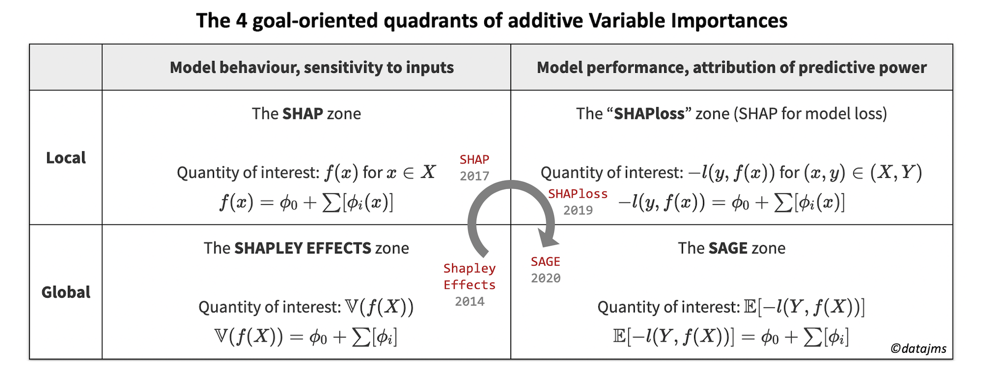
These local vs global scopes and sensitivity vs predictive power metrics define a 2 by 2 goal-oriented matrix. Each quadrant has been named by the importance measure which is theoretically “optimal” for its quantity of interest. The equations are a simplified version of the additive breakdown of each quantity of interest (see below for more precise formulation).

To be more specific, let’s introduce some notations. Suppose that from your variables \(X = (X_1, X_2, …, X_d)\), you try to predict \(Y\) with your model \(f(X) \in \mathbb{R} \) minimizing the loss function \(l(y, f(x))\). \(y\) and \(x\) refer to one data point while \(Y\) and \(X\) are at population level (random variables). \(\mathbb{E}\) and \(\mathbb{V}\) respectively denotes the expectation (the “average”) and the variance of a variable.

The 4 purpose-oriented quadrants

Let’s have a look at the 4 quadrants and the different problems they solve. The precise definition of their optimal solution is given in the next part. We will make this journey in chronological order because it tells a good story on how two different research communities finally meet!

The SHAPLEY EFFECTS zone

Context

Improving Sobol indices (1993¹), Owen introduced an importance measure in 2014², that has been developed and named “shapley effects” by Song et al. in 2016³ (see also further work and numerical experiment by Iooss et al. in 2017⁴). Coming from the field of Sensitivity Analysis and Uncertainty Quantification, it aims at quantifying how much the output of a model \(f\) (for example a computer simulation of a set of complicated equations) depends on the \(X\) input parameters. Shapley effects are also totally relevant in machine learning where it focuses on how much the variations of the learned model \(f\) would rely on the variables \(X\).

The choice of a Quantity of interest

The quantity of interest is \(\mathbb{V}(f(X))\). Variance is a natural choice to quantify variations and usually more tractable than a potential alternative \(\mathbb{E}(|f(X)-\mathbb{E}(f(X))|)\) never encountered in practice. Note that in Sensitivity Analysis community, indices are usually normalized by the total variance, so that all Variable Importances sum to 1 (or “near” 1 with Sobol Indices).

By looking at the 4 quadrants, a question arises: why not choosing \(\mathbb{E}(f(X))\) as a quantity of interest? It is definitely global. However it is not relevant to account for variations: positive and negative variations would annihilate into a 0 global contribution.

Let’s move on to 2017, the start the Lundberg saga in the machine learning community.

The SHAP zone

Context

Designed and implemented by Lundberg in 2017⁵, shap a has local sensitivity focus. Note that although published in a machine learning conference, shap does not involve a \(Y\) target or any learning of the model \(f\). That’s why I was able to apply it to a non-learned, expert based algorithm for Covid-19 patient orientation. However, it is strongly suited to machine learning community, because of its fast model-specific implementations.

The choice of a Quantity of interest

The quantity of interest sticks to the most natural choice: \(f(x)\) for \(x \in X\). Unlike the global scope, having both positive and negative contributions makes sense here. Knowing the direction of variation is totally relevant and allow nice visual exploration of shap values (implemented in the shap package).

The SHAPloss zone

Context

Published in Nature in 2020⁶ (but pre-print in 2019), Lundberg et al. presented an innovation! Although the paper focuses on tree-based models, a new idea has been proposed: using shap to breakdown the model error into a feature contributions (see §2.7.4 and Figure 5 of the paper), making it very useful for supervised performance monitoring of a model in production. I’ve made up the name SHAPloss to insist on the different goal achieved, although implementation is done inside shap package by changing only the model_output argument in TreeExplainer.

The choice of a Quantity of interest

The quantity of interest is the local loss \(-l(y, f(x))\) for \((x, y) \in (X, Y)\). Note that \(l\) could naturally be the logloss for a classification problem, while being the MSE for a regression. The minus sign is added so that a large positive contribution \(\phi_i\) means a feature which increases the performance a lot (= decrease a lot the model loss \(l\)).

The SAGE zone

Context

With a preprint submitted in April 2020⁷, Covert, Lundberg et al. introduce SAGE (Shapley Additive Global importancE), a solution of the global formulation of SHAPloss and efficient ways of computing it. Note that the paper goes far beyond a simple local to global generalization of SHAPloss, but it also includes a review of existing importance methods and introduces a theoretical universal predictive power. Furthermore, the SAGE paper makes a clear reference to what we called the Shapley Effects zone, explaining how SAGE differs in its goal. In some ways, it closes the 4-quadrant loop we have explored.

The choice of a Quantity of interest

The quantity of interest is \(\mathbb{E}[-l(Y, f(X))]\), a natural aggregation of the local SHAPloss formulation. Unlike the SHAP to Shapley Effects transition, taking the raw expectation works here. This is because there is almost no positive-negative annihilation, for adding a variable usually does not increase the loss.

A shapley solution for each quadrant

Now that the purpose and its quantity of interest have been set, Shapley values ⁸ theory offers optimal solutions given desirable properties for each quadrant. Let’s introduce Shapley values first and see how it applies to the various quantities of interest.

Shapley values

The Shapley value \(\phi_i^Q\) is an attribution method which “fairly” shares the quantity of interest \(Q(P_d)\) obtained by the coalition \(P_d = \{1, 2, .., d\}\) between each entity \(i \in P_d\). \(Q(u)\) is a function returning the quantity of interest of coalition \(u\). A coalition is a set of entity \(i\): there are \(2^d\) possible coalitions, including \(\emptyset\) and \(P_d\). Finally, let’s denote by \(S_i^d\) the set of all possible coalitions which do not contain the entity \(i\).

The Shapley values \(\phi_i^Q\) are the only quantity weighting which satisfies 5 desirable properties (check §3.1 of SAGE paper⁷ for their meaning) named symmetry, linearity, monotonicity, dummy and finally efficiency, which we write here:
\(Q(P_d)=Q(\emptyset) + \sum[\phi_i^Q]\)

There is a lot to talk about concerning the formula of this Shapley values. But it is slightly off-topic and I would rather focusing on how this Shapley idea is applied to the 4 quadrants. You can see the formula as a footnote⁹.

Application to feature attribution

Using Shapley values in our context means that the \(i\) entities will be the \(X_i\) variables. The two remaining tasks are to choose the quantity of interest \(Q\) and to define \(f\) for each coalition of variables \(u\). The solution chosen for our 4-quadrant is to take the expectation along missing variables: \(f_u(x) = \mathbb{E}(f(X|X_u=x_u))\). For more information, see an example for 2 variables in footnote¹⁰ and details in the SAGE paper.

The 4 quantities of interest translates into 4 \(Q(u)\) functions, which lead to the 4 names of the quadrants: the Variable Importance methods which have desirable properties!

Let’s rewrite the 2 by 2 matrix with more precise quantities of interest \(Q(u)\), which are functions of \(f\) and of all feature coalitions \(u\) (\(u \in \{\emptyset, \{X_1\},\{X_2\}, .., \{X_1, X_2\}, .. \}\)).

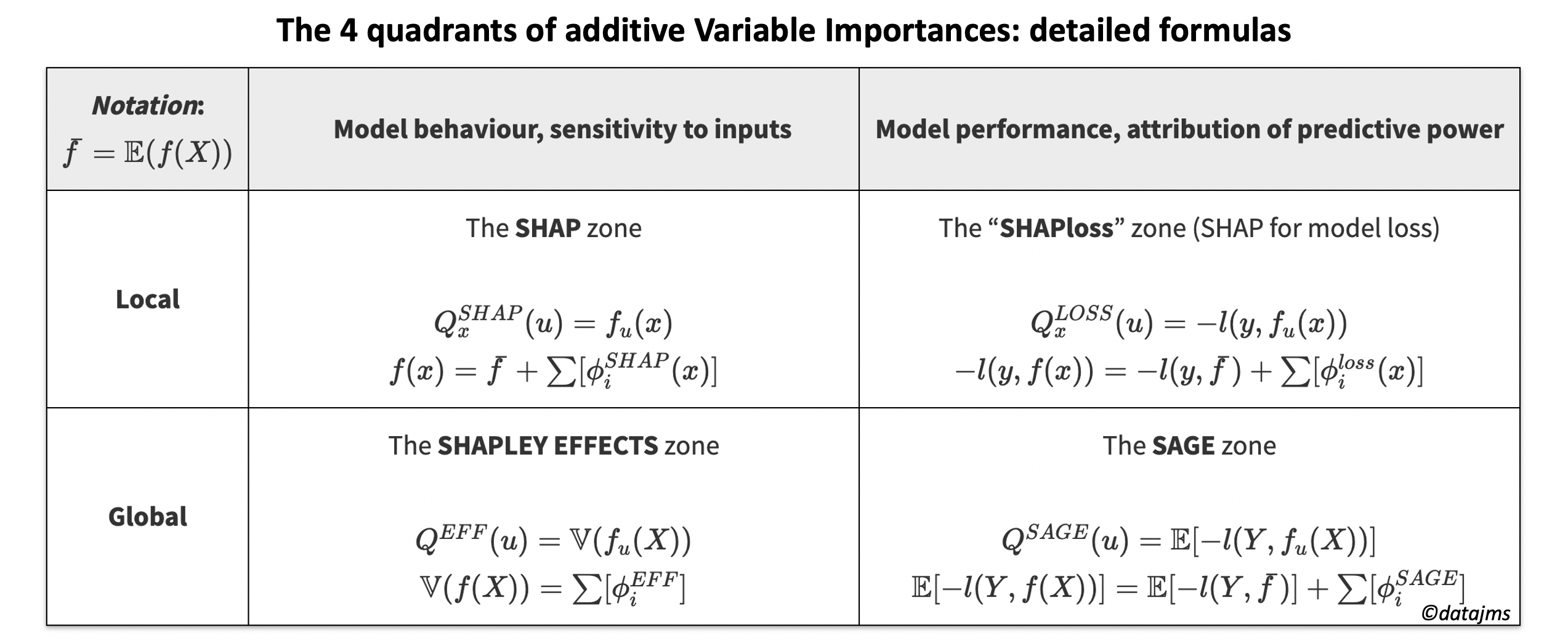
The four Shapley values \(\phi_i^{SHAP}(x)\), \(\phi_i^{LOSS}(x)\), \(\phi_i^{EFF}\) and \(\phi_i^{SAGE}\) are the “optimal” solutions of each quadrant. Note that there are 2 links between those values:

• \(\phi_i^{SAGE} = \mathbb{E}[\phi_i^{LOSS}(x)] \)
• Potentially, if the loss function \(l\) is the MSE, we have \(\phi_i^{EFF} = \phi_i^{SAGE} \) with \(Y = f(X)\).

Future perspectives

We have just seen that “optimal” solutions have been defined and that implementations are available, for each quadrant. So, has the full story being told ?

On the one hand, I think the field of additive importance measures has reached a maturity milestone by optimally filling the 4 quadrants and therefore closing the loop. Until the SAGE article, I was not aware of any clear formalization of the links between Sensitivity Analysis and the predictive power importance.

On the other hand, there is still room for enhancements concerning Variable Importance and feature attribution, concerning both a better use of these techniques and exploring value outside of this perimeter:

• Towards a better use of the methods in the quadrants:
  • Diffusion of SHAPloss in data science community: Although SHAP has had a very fast adoption rate in the data science community in about 2 years, SHAPloss has currently stayed under the radar (except from an inspirational notebook by Hall). I see value for supervised (when ground-truth labels are known) performance monitoring of a model in production.
  • Improvements of computation efficiency: These methods are computationally intensive and can rapidly become un-tractable, except for tree-based models. Improvements in implementation and statistical estimation could improve the usability (see recent work¹¹).
• Beyond the 2 by 2 matrix:
  • Fairness-based quantities of interest: Why not imagining other columns? Understanding the model behaviour and the model performance are the first important steps. But responsible data science also include a bias and fairness monitoring when relevant. Theoretically, it seems possible to chose a fairness-based relevant quantity of interest \(Q(u)\) and build its Shapley value to see how “unfairness” would be divided between features. Lundberg opens the way with the demographic parity metrics, which cleverly stays within the SHAP zone.
  • Explore non additive feature attribution methods. Should it be done with a multiplicative breakdown or with totally different re-weighting methods¹², quantifying how much a quantity of interest rely on the input features is still broad research and practice field.

Take-away messages

I hope that this post has:

• Enlightened your understanding of the different goals and scopes of Variable Importances.
• Convinced you that the field of additive importance measures is definitely more mature than ever since Sobol started it in the 1990s.
• Made you think about the most effective quadrant to choose, given your purpose.

Interested in an experiment with results and code for SHAP and SHAPLEY EFFECTS zone ? You can check my article on Variable importance for the Covid-19 patient orientation algorithm. Furthermore, you can check the SAGE paper⁷ for more examples of non optimal but computationally light methods and how they fit in the 2 by 2 matrix.

Congrats to Scott Lundberg for having pioneered the way in so many topics and ideas in just a few years!

---

1. Sobol, I. M. (1993). Sensitivity estimates for nonlinear mathematical models. Mathematical modelling and computational experiments, 1(4), 407-414. Incidentally, the only online version I found is a photocopy, annotated by hand by I. M. Sobol himself, sent to Andrea Saltelli, a well known researcher in Sensitivity Analysis. ↩︎

2. Owen, A. B. (2014). Sobol’indices and Shapley value. SIAM/ASA Journal on Uncertainty Quantification, 2(1), 245-251. ↩︎

3. Song, E., Nelson, B. L., & Staum, J. (2016). Shapley effects for global sensitivity analysis: Theory and computation. SIAM/ASA Journal on Uncertainty Quantification, 4(1), 1060-1083. ↩︎

4. Iooss, B., & Prieur, C. (2019). Shapley effects for sensitivity analysis with correlated inputs: comparisons with Sobol’indices, numerical estimation and applications. International Journal for Uncertainty Quantification, 9(5). ↩︎

5. Lundberg, S. M., & Lee, S. I. (2017). A unified approach to interpreting model predictions. In Advances in neural information processing systems (pp. 4765-4774). ↩︎

6. Lundberg, S. M., Erion, G., Chen, H., DeGrave, A., Prutkin, J. M., Nair, B., Katz, R., Himmelfarb, J., Bansal, N., & Lee, S. I., (2020). From local explanations to global understanding with explainable AI for trees. Nature machine intelligence, 2(1), 2522-5839. ↩︎

7. Covert, I., Lundberg, S., & Lee, S. I. (2020). Understanding Global Feature Contributions Through Additive Importance Measures. arXiv preprint arXiv:2004.00668. ↩︎

8. Shapley, L. S. (1953). A value for n-person games. Contributions to the Theory of Games, 2(28), 307-317. ↩︎

9. \( \phi_i^Q = \sum_{u \in S_i^d}(\alpha_{|u|} * [Q(u \cup { i}) - Q(u)]) \text{ , where } \alpha_{k} = \frac{1}{d} {\binom{d-1}{k}}^{-1} \) ↩︎

10. Let’s suppose we have 2 features, then there are 4 coalitions to form: \(f_\emptyset((x_1, x_2)) = \mathbb{E}(f(X))\), \(f_1(x_1, x_2) = \mathbb{E}(f(X | X_1=x_1))\), \(f_2(x_1, x_2) = \mathbb{E}(f(X | X_2=x_2))\) and \(f_{1,2}(x_1, x_2) = \mathbb{E}(f(X | X_1=x_1, X_2=x_2)) = f(x_1, x_2)\) ↩︎

11. This recent preprint by Plischke et al. improves Shapley effects computation by several orders of magnitude: Plischke, E., Rabitti, G., & Borgonovo, E. (2020). Computing Shapley Effects for Sensitivity Analysis. arXiv preprint arXiv:2002.12024. ↩︎

12. Bachoc, F., Gamboa, F., Loubes, J. M., & Risser, L. (2018). Entropic Variable Boosting for Explainability & Interpretability in Machine Learning. ↩︎